

필터드 인덱스 부작용
https://www.sql.kiwi/2014/06/filtered-index-side-effect/
filtered index 해결하기 힘든 문제가 있다.
update(insert update delete merge 모두를 그냥 update 라 한다)에서 narrow 와 wide 플랜을 선택할 때 traceflag를 이용하지 말고 top 절과 optimize for 를 이용하는 방법도 있다.
-- All qualifying rows will be deleted
DECLARE @Rows bigint = 9223372036854775807;

-- Optimize the plan for deleting 100 rows
DELETE TOP (@Rows)
FROM dbo.[Data]
OUTPUT
    Deleted.RowID,
    Deleted.SomeValue,
    Deleted.StartDate,
    Deleted.CurrentFlag
WHERE StartDate = CONVERT(date, '20140106', 112)
OPTION (OPTIMIZE FOR (@Rows = 100));
CTE 를 쓰면 어떤 잇점이 있을까?
쿼리 가독성과 대상의 확인 select 가 하나의 쿼리로 할 수 있다. (select 만 실행 가능하다. )
옵티마이저가 이상한 플랜 만들수 있으니 성능 테스트 해보고 쓰자~
WITH
    LastRowPerDay AS
    (
        SELECT
            D.CurrentFlag
        FROM dbo.[Data] AS D
        WHERE
            D.RowID =
            (
                SELECT MAX(D2.RowID)
                FROM dbo.[Data] AS D2
                WHERE D2.StartDate = D.StartDate
            )
    )
UPDATE LastRowPerDay
SET CurrentFlag = 'true';


-- VS

UPDATE D
SET CurrentFlag = 'true'
FROM dbo.[Data] AS D
WHERE D.RowID = (
    SELECT MAX(D2.RowID)
    FROM dbo.[Data] AS D2
    WHERE D2.StartDate = D.StartDate
);
An Unexpected Side-Effect of Adding a Filtered Index
Adding a filtered index can have surprising side-effects on existing queries, even where it seems the new filtered index is completely unrelated.
www.sql.kiwi
An Unexpected Side-Effect of Adding a Filtered Index

Adding a filtered index can have surprising side-effects on existing queries, even where it seems the new filtered index is completely unrelated. This post looks at an example affecting DELETE statements that results in poor performance and an increased risk of deadlock.
Note: The behaviour described in this article is current as of November 2024.
(tested on SQL Server 2022 CU15)
Test Environment
The following table will be used throughout this post:
CREATE TABLE dbo.[Data]
(
    RowID integer IDENTITY NOT NULL,

    CONSTRAINT PK_Data_RowID
        PRIMARY KEY CLUSTERED (RowID),

    SomeValue integer NOT NULL,
    StartDate date NOT NULL,
    CurrentFlag bit NOT NULL,
    Padding char(50) NOT NULL
        DEFAULT REPLICATE('ABCDE', 10)
);
This next statement creates 499,999 rows of sample data:
INSERT dbo.[Data]
    WITH (TABLOCKX)
(
    SomeValue,
    StartDate,
    CurrentFlag
)
SELECT
    SomeValue = CONVERT(integer, RAND(n) * 1e6) % 1000,
    StartDate = DATEADD(DAY, (N.n - 1) % 31, CONVERT(date, '20140101', 112)),
    CurrentFlag = CONVERT(bit, 0)
FROM dbo.Numbers AS N
WHERE
    N.n >= 1
    AND N.n < 500 * 1000;
That uses a Numbers table as a source of consecutive integers from 1 to 499,999. In case you do not have one of those in your test environment, the following code can be used to efficiently create one containing integers from 1 to 1,000,000:
WITH
    N1 AS (SELECT N1.n FROM (VALUES (1),(1),(1),(1),(1),(1),(1),(1),(1),(1)) AS N1 (n)),
    N2 AS (SELECT L.n FROM N1 AS L CROSS JOIN N1 AS R),
    N3 AS (SELECT L.n FROM N2 AS L CROSS JOIN N2 AS R),
    N4 AS (SELECT L.n FROM N3 AS L CROSS JOIN N2 AS R),
    N AS (SELECT ROW_NUMBER() OVER (ORDER BY n) AS n FROM N4)
SELECT
    -- Destination column type integer NOT NULL
    ISNULL(CONVERT(integer, N.n), 0) AS n
INTO dbo.Numbers
FROM N
OPTION (MAXDOP 1);

ALTER TABLE dbo.Numbers
ADD CONSTRAINT PK_Numbers_n
PRIMARY KEY (n)
WITH (SORT_IN_TEMPDB = ON, MAXDOP = 1);
The basis of the later tests will be to delete rows from the test table for a particular StartDate. To make the process of identifying rows to delete more efficient, add this nonclustered index:
CREATE NONCLUSTERED INDEX
    IX_Data_StartDate
ON dbo.[Data]
    (StartDate);
The sample data
Once those steps are completed, the data will look like this:
SELECT TOP (100)
    D.RowID,
    D.SomeValue,
    D.StartDate,
    D.CurrentFlag,
    D.Padding
FROM dbo.[Data] AS D
ORDER BY
    D.RowID;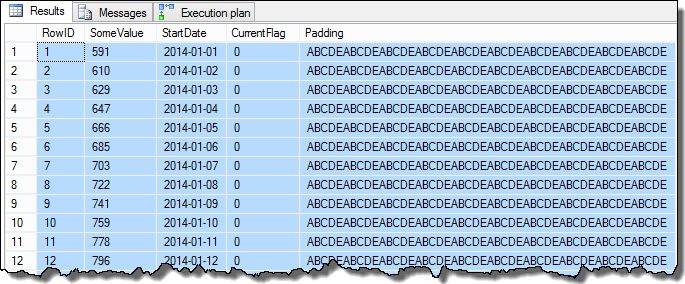
The SomeValue column data may be slightly different due to the pseudo-random generation, but this difference is not important. Overall, the sample data contains 16,129 rows for each of the 31 StartDate dates in January 2014:
SELECT
    D.StartDate,
    NumRows = COUNT_BIG(*)
FROM dbo.[Data] AS D
GROUP BY
    D.StartDate
ORDER BY
    D.StartDate;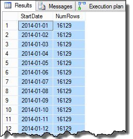
The last step we need to perform to make the data somewhat realistic, is to set the CurrentFlag column to true for the highest RowID for each StartDate. The following script accomplishes this task:
WITH
    LastRowPerDay AS
    (
        SELECT
            D.CurrentFlag
        FROM dbo.[Data] AS D
        WHERE
            D.RowID =
            (
                SELECT MAX(D2.RowID)
                FROM dbo.[Data] AS D2
                WHERE D2.StartDate = D.StartDate
            )
    )
UPDATE LastRowPerDay
SET CurrentFlag = 'true';
The execution plan for this update features a Segment-Top combination to efficiently locate the highest RowID per day:
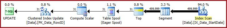
Notice how the execution plan bears little resemblance to the written form of the query. This is a great example of how the optimizer works from the logical SQL specification, rather than implementing the SQL directly. In case you are wondering, the Eager Table Spool in that plan is required for Halloween Protection.
Deleting a Day of Data
With the preliminaries completed, the task at hand is to delete rows for a particular StartDate. This is the sort of query you might routinely run on the earliest date in a table, where the data has reached the end of its useful life.
Taking 1 January 2014 as our example, the test delete query is simple:
DELETE FROM
    dbo.[Data]
WHERE
    1 = 1
    AND StartDate = CONVERT(date, '20140101', 112);
The execution plan is likewise pretty simple, though worth looking at in a bit of detail:
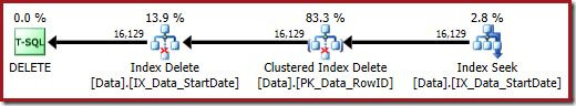
Note: If you don’t see a separate Index Delete operator, try changing the maximum memory available to SQL Server to around 4GB. You may then need to repopulate the test table or clear the plan cache to get the desired plan shape.
Plan analysis
The Index Seek on the far right uses the nonclustered index to find rows for the specified StartDate value. It returns just the RowID values it finds, as the operator tooltip confirms:

If you are wondering how the StartDate index manages to return the RowID, remember that RowID is the unique clustered index for the table, so it is automatically included in the StartDate nonclustered index.
The next operator in the plan is the Clustered Index Delete. This uses the RowID value found by the Index Seek to locate rows to remove.
The final operator is an Index Delete. This removes rows from the nonclustered index IX_Data_StartDate that are related to the RowID removed by the Clustered Index Delete. To locate these rows in the nonclustered index, the query processor needs the StartDate (the key for the nonclustered index).
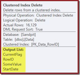
Remember the original Index Seek did not return the Start Date, just the RowID. So how does the query processor get the StartDate for the index delete? In this particular case, the optimizer might have noticed that the StartDate value is a constant and optimized it away, but this is not what happened. The answer is that the Clustered Index Delete operator reads the StartDate value for the current row and adds it to the stream. Compare the Output List of the Clustered Index Delete shown below, with that of the Index Seek just above:

It might seem surprising to see a Delete operator reading data, but this is the way it works. The query processor knows it will have to locate the row in the clustered index in order to delete it, so it might as well defer reading columns needed to maintain nonclustered indexes until that time, if it can.
Adding a Filtered Index
Now imagine someone has a crucial query against this table that is performing badly. The helpful DBA performs an analysis and adds the following filtered index:
CREATE NONCLUSTERED INDEX
    FIX_Data_SomeValue_CurrentFlag
ON dbo.[Data]
    (SomeValue)
INCLUDE
    (CurrentFlag)
WHERE
    CurrentFlag = 'true';
The new filtered index has the desired effect on the problematic query and everyone is happy. Notice that the new index does not reference the StartDate column at all, so we do not expect it to affect our day-delete query at all.
Deleting a day with the filtered index in place
We can test that expectation by deleting data for a second time:
DELETE FROM
dbo.[Data]
WHERE
1 = 1
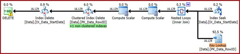
AND StartDate = CONVERT(date, '20140102', 112);Suddenly, the execution plan has changed to a parallel Clustered Index Scan:

If you don’t see a parallel plan, ensure your cost threshold for parallelism is set to the default value of 5 for these tests.
Notice there is no separate Index Delete operator for the new filtered index. The optimizer has chosen to maintain this index inside the Clustered Index Delete operator. This is highlighted in Plan Explorer as shown above (“+1 non-clustered indexes”) with full details in the tooltip:
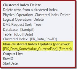
If the table is large, this change to a parallel scan might be very significant. What happened to the nice Index Seek on StartDate, and why did a completely unrelated filtered index change things so dramatically?
Finding the problem
The first clue comes from looking at the properties of the Clustered Index Scan:
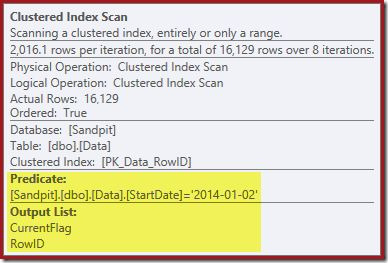
As well as finding RowID values for the Clustered Index Delete operator to delete, this operator is now reading CurrentFlag values. The need for this column is unclear, but it does at least begin to explain the decision to scan: The CurrentFlag column is not part of our StartDate nonclustered index.
We can confirm this by rewriting the delete query to force the use of the StartDate nonclustered index:
DELETE FROM D
FROM dbo.[Data] AS D
WITH (INDEX(IX_Data_StartDate))
WHERE
1 = 1
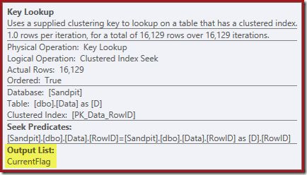
AND StartDate = CONVERT(date, '20140103', 112);The execution plan is closer to its original form, but it now features a Key Lookup:
The Key Lookup properties confirm this operator is retrieving CurrentFlag values:
You might also have noticed the warning triangles in the last two plans. These are missing index warnings:
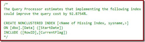
This is further confirmation that SQL Server would like to see the CurrentFlag column included in the nonclustered index. The reason for the change to a parallel Clustered Index Scan is now clear: The query processor decides that scanning the table will be cheaper than performing the Key Lookups.
Yes, but why?
This is all very weird. In the original execution plan, SQL Server was able to read extra column data needed to maintain nonclustered indexes at the Clustered Index Delete operator. The CurrentFlag column value is needed to maintain the filtered index, so why does SQL Server not just handle it in the same way?
The short answer is that it can, but only If the filtered index is maintained in a separate Index Delete operator. We can force this for the current query using undocumented trace flag 8790. Without this trace flag, the optimizer chooses whether to maintain each index in a separate operator or as part of the base table operation.
-- Forced wide update plan
DELETE FROM
dbo.[Data]
WHERE
1 = 1
AND StartDate = CONVERT(date, '20140105', 112)
OPTION
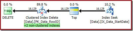
(QUERYTRACEON 8790);The execution plan is back to seeking the StartDate nonclustered index:

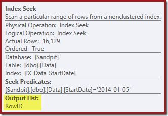
The Index Seek returns just RowID values (no CurrentFlag):
The Clustered Index Delete now reads the columns needed to maintain the nonclustered indexes, including CurrentFlag:
This data is eagerly written to a table spool, which is replayed for each index that needs maintaining. Notice also the explicit Filter operator before the Index Delete operator for the filtered index.
Another pattern to watch out for
This problem does not always result in a table scan instead of an index seek. To see an example of this, add another index to the test table:
CREATE NONCLUSTERED INDEX
    IX_Data_SomeValue_CurrentFlag
ON dbo.[Data]
    (SomeValue, CurrentFlag);
Note this index is not filtered, and does not involve the StartDate column. Now try a day-delete query again:
DELETE FROM
    dbo.[Data]
WHERE
    1 = 1
    AND StartDate = CONVERT(date, '20140104', 112);
The optimizer now comes up with this monster:

This query plan has a high surprise factor, but the root cause is the same. The CurrentFlag column is still needed, but now the optimizer chooses an index intersection strategy to get it instead of a table scan. Using the trace flag forces a per-index maintenance plan and sanity is once again restored (the only difference is an extra spool replay to maintain the new index):

Only Filtered Indexes Cause This
This issue only occurs if the optimizer chooses to maintain a filtered index in a Clustered Index Delete operator. Non-filtered indexes are not affected, as the following example shows. The first step is to drop the filtered index:
DROP INDEX
    FIX_Data_SomeValue_CurrentFlag
ON dbo.[Data];
Now we need to write the query in a way that convinces the optimizer to maintain all the indexes in the Clustered Index Delete. My choice for this is to use a variable and a hint to lower the optimizer’s row count expectations:
-- All qualifying rows will be deleted
DECLARE @Rows bigint = 9223372036854775807;

-- Optimize the plan for deleting 100 rows
DELETE TOP (@Rows)
FROM dbo.[Data]
OUTPUT
    Deleted.RowID,
    Deleted.SomeValue,
    Deleted.StartDate,
    Deleted.CurrentFlag
WHERE StartDate = CONVERT(date, '20140106', 112)
OPTION (OPTIMIZE FOR (@Rows = 100));
The execution plan is:
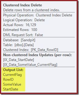
Both nonclustered indexes are maintained by the Clustered Index Delete:
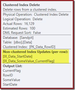
The Index Seek returns only the RowID:

The columns needed for the index maintenance are retrieved internally by the delete operator. These details are not exposed in show plan output (so the output list of the delete operator would be empty). I added an OUTPUT clause to the query to show the Clustered Index Delete once again returning data it did not receive on its input:
Final Thoughts
This is a tricky limitation to work around. On the one hand, we generally do not want to use undocumented trace flags in production systems.
The natural ‘fix’ is to add the columns needed for filtered index maintenance to all nonclustered indexes that might be used to locate rows to delete. This is not a very appealing proposition, from a number of points of view. Another alternative is to just not use filtered indexes at all, but that is hardly ideal either.
My feeling is that the query optimizer ought to consider a per-index maintenance alternative for filtered indexes automatically, but its reasoning appears to be incomplete in this area right now (and based on simple heuristics rather than properly costing per-index/per-row alternatives).
To put some numbers around that statement, the parallel clustered index scan plan chosen by the optimizer came in at 5.5 units in my test. The same query with the trace flag estimates a cost of 1.4 units. With the third index in place, the parallel index-intersection plan chosen by the optimizer had an estimated cost of 4.9, whereas the trace flag plan came in at 2.7 units (all tests on SQL Server 2014 RTM CU1 build 12.0.2342 under the 120 cardinality estimation model and with trace flag 4199 enabled).
I regard this as behaviour that should be improved. You can vote to agree with me on this Azure Feedback item.
Thanks for reading.


